Working with Simplex Noise
Recently, I’ve been getting into procedural content generation (PCG), with the end-goal of procedurally generating entire worlds. When you consider the fact that my artistic abilities are incredibly lacking, it only makes sense that I would consider having algorithms make things for me. Add in the coolness (read: geek) factor, and it’s a wonder that I actually managed to get my other work done before plunging head-first into some PCG experimentation.
Being new to the world of PCG, I decided to do some research. The first thing I learned was that I would need a decent noise implementation to generate random values. Ken Perlin seems to be the name in noise functions. He made his original algorithm for Perlin noise while working on the original Tron, and he released an improved noise function, simplex noise, back in 2001. These noise functions produce pseudo-random smooth gradients. This noise results in a very natural appearance, so you might have come across it if you’ve done work with terrain heightmaps or particle effects.
For my project, I decided to use simplex noise, since it’s less computationally expensive and gives better results. I’m not going to go into the details of the algorithm– an excellent paper by Stefan Gustavson already does the job far better than I ever could. But for a high-level overview, it’s enough to know that the algorithm uses something known as a simplex grid to add nearby values and produce numbers between -1 and 1 that look linearly-interpolated like classic Perlin noise.
Simplex noise is a complicated beast. It’s a straight-up math algorithm involving simplices and is designed to be implemented in hardware. To make matters worse, Ken Perlin’s sample implementation (appendix B) is near-indecipherable for the common mind. Thankfully, Gustavson comes to the rescue again by providing implementations in C and C++, as well as in Java, Lua, and GLSL. The implementations provide noise values for up to four dimensions (generally used as three dimensions + time).
With all of the hard work done for us, we really just need to figure out how to use the provided simplex noise functionality. The various implementations provide a noise function that takes a coordinate and returns a floating-point noise value between -1 and 1, inclusive, where coordinates that are close to each other have similar values. To make a general-purpose heightmap, we need to fill an MxN matrix with luminosity (light) values, between 0 and 255. Let’s normalize the simplex noise to our light range and populate our array:
for(i = 0; i < M; ++i):
    for(j = 0; j < N; ++j):
        luminance[i][j] = (simplex_noise(i, j) + 1) / 2.0  * 255.0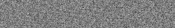
That’s all we need, right? Well, it turns out that this produces an image that doesn’t look much better than white noise (that awful static you get on you TV when it doesn’t get a proper signal). How can we smooth this out? First recall that the term “noise” is related to sound, and sound is just a wave. So to simplify matters, we can think of our noise as a wave. Our current noise changes quickly from one value to another. In wave terms, this means that our noise has a very high frequency. What we want is noise with a low-frequency, so that values change gradually.
From physics, we know that, for a wave, \(\textrm{frequency} = \frac{\textrm{velocity}}{\textrm{wavelength}}\). We don’t have a convenient method of changing the wave length, so this means that we have to change our noise’s velocity. But what is the current velocity of our noise? Recall that \(\textrm{velocity} = \frac{\textrm{distance}}{\textrm{time}}\). In the sample code, i and j (the distance) are increased by one in each (time) step, so the velocity is one. In order to decrease our frequency, we need to decrease our velocity, and to do that, we need to scale the values that we send to our noise function by some small value:
scale = .007
for(i = 0; i < M; ++i):
   for(j = 0; j < N; ++j):
       luminance[i][j] = (simplex_noise(i * scale, j * scale) + 1) / 2.0 * 255.0
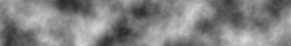
It turns out that we need to use a very small scale in order to produce good smooth noise like the type shown above. I use .007, because I like to imagine a very small James Bond making things smooth and suave, but other values around .01 work well for my project. You’ll have to experiment with the scale to see what suits your purposes best.
So now we have the smooth noise shown above, but it still seems kind of boring and unsatisfying. Instead of purely smooth noise we want something a bit more chaotic and organic. To get this, we’re going to need to use another technique: fractal Brownian motion. This method works by using our noise function for multiple iterations, decreasing the amplitude and increasing the frequency in each successive iteration. It then sums all these iterations together and takes the average. From there, we can normalize the value and add the result to our array.
def sumOcatave(num_iterations, x, y, persistence, scale, low, high):
    maxAmp = 0
    amp = 1
    freq = scale
    noise = 0

    #add successively smaller, higher-frequency terms
    for(i = 0; i < num_iterations; ++i):
        noise += simplex_noise(x * freq, y * freq) * amp
        maxAmp += amp
        amp *= persistence
        freq *= 2

    #take the average value of the iterations
    noise /= maxAmp

    #normalize the result
    noise = noise * (high - low) / 2 + (high + low) / 2

    return noise

def main():
    scale = .007
    for(i = 0; i < M; ++i):
        for(j = 0; j < N; ++j):
            luminance[i][j] = sumOctave(16, i, j, .5, scale, 0, 255)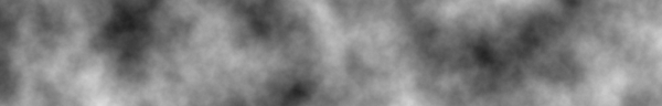
This finally gets us the results we want. In the above code, each iteration is called an octave, because it is twice the frequency of the iteration before it, just like musical notes double in frequency as you go up an octave. The amplitude is the relative importance of the octave in the sum of the octaves, and persistence is is the scale factor in each iteration. We want the amplitude to decrease, so our persistence is less than 1. Additionally, the above method allows us to scale our noise from low to high instead of just 0 to 255.
So we have some good-looking noise that we can apply to textures or make a heightmap, etc. But using fractal Brownian motion isn’t the only way to get cool results out of noise. By using different techniques, you can use basic simplex noise to procedurally generate textures that look remarkably like dust, fire, marble, or even wood. You can try to figure these out on your own, or look around on the internet (note: techniques for using Perlin noise will pretty much get the same results with simplex noise). If you want to learn more, the links throughout the article, and below should help you.
Update
It turns out that Simplex Noise is patented. OpenSimplexNoise is a free alternative.
Resources
Clojure implementation of layered noise functions using OpenSimplexNoise
Java, Lua, GLSL implementations
The more technical paper by Ken Perlin
An article explaining Perlin noise, octaves, and fun textures